“The Solow–Swan model, or exogenous growth model, is an economic model of long-run economic growth. It attempts to explain long-run economic growth by looking at capital accumulation, labor or population“
Wikipedia
Nudel sought to test ChatGPT’s ability to build an economic model by asking:
“Build an excel file that models Solow-Swan economic growth”
Like many ChatGPT outputs, the result was interesting, but flawed:
To build an Excel model for the Solow-Swan economic growth model, we'll create a simple spreadsheet that calculates economic outputs over time based on initial conditions and assumptions of the model. The Solow-Swan model typically uses parameters like savings rate, depreciation rate, population growth rate, and the rate of technological progress. Here's how we can structure the model:
1. Parameters:
( s ): Savings rate
( n ): Population growth rate
( g ): Technological growth rate
( delta ): Depreciation rate
( alpha ): Capital's share of income (elasticity of output with respect to capital)
2. Initial Conditions:
( K_0 ): Initial capital stock
( L_0 ): Initial labor force
( A_0 ): Initial level of technology
( Y_0 ): Initial output, calculated as ( Y_0 = A_0 imes K_0^alpha imes L_0^{1-alpha} )
3. Yearly Calculations:
( A_{t} = A_{t-1} imes (1 + g) ): Technology next year
( L_{t} = L_{t-1} imes (1 + n) ): Labor force next year
( K_{t} = (1 - delta) imes K_{t-1} + s imes Y_{t-1} ): Capital stock next year
( Y_{t} = A_{t} imes K_{t}^alpha imes L_{t}^{1-alpha} ): Output next year
4. Output for Analysis:
Per capita output: ( y_t = rac{Y_t}{L_t} )
Capital per worker: ( k_t = rac{K_t}{L_t} )
Let's go ahead and set up these calculations in an Excel file. I'll create the initial structure and formulas based on typical economic growth parameters. After that, I can share the file with you.
ChatGPT 4, May 2024
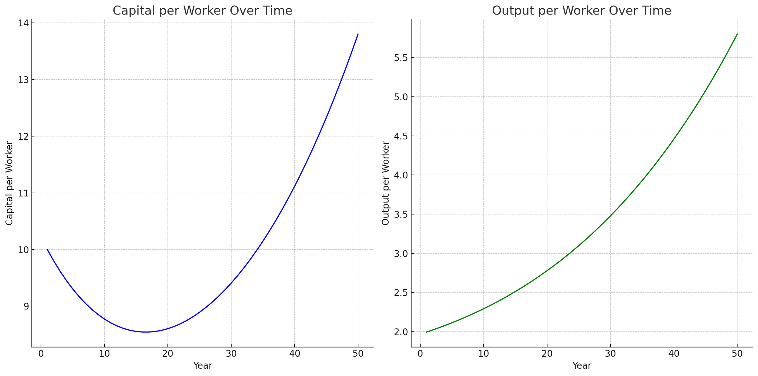
Nudel then asked ChatGPT to output plots from the Excel files resulting in the graphs above. The hockey-stick curve shown is distinctly different to the relationship expected of the Solow-Swan model whereby marginal gains in capital per capita decrease as an economy matures.
ChatGPT explained the results of its outputs from Excel as follows:
The appearance of a "hockey stick" relationship in the graph of capital per capita over time can initially seem counterintuitive given the principle of diminishing returns to capital. However, this visual trend can be explained by several factors related to the parameters and dynamics of the Solow-Swan model:
1. Accumulation Phase: Early in the development process, significant increases in capital per worker can occur because the economy is starting from a lower base of capital. This phase often shows rapid growth as initial investments yield high returns due to relatively scarce capital.
2. Compound Growth: Even with diminishing returns to capital, as long as the savings rate remains constant and above the combined rates of population growth and depreciation, the economy can still accumulate capital. The model incorporates reinvestment of a portion of output, which compounds over time, leading to a rapid increase in capital stock initially.
3. Technological Growth: The model you've seen also includes technological progress, which enhances the productivity of both capital and labor. Technological growth can offset some of the diminishing returns to capital by effectively increasing the output generated from existing levels of capital and labor.
4. Transition to Steady State: Over a longer period, the economy should approach a steady state where the rate of capital accumulation aligns more closely with the rates of population growth and depreciation. In the steady state, increases in capital per worker taper off, and any further growth in output per worker is primarily due to technological advancements rather than capital deepening.
The "hockey stick" growth might be more pronounced depending on the initial conditions (like a very low initial capital per worker) and the specific parameter values for savings, depreciation, population growth, and technological progress. If the model's assumptions were altered (e.g., a lower savings rate or higher depreciation), the curve might flatten earlier or rise less steeply. This shape underscores how sensitive the model's outcomes can be to its input parameters.

